Control Systems
Table of Contents
- 1 Intro to Control Systems
- 2 Open Loop-and Closed Loop Control
- 3 Feedback
- 4 Block Diagrams
- 5 Transfer Functions
- 6 Time Response Analysis
- 7 Response of a First Order System
- 8 Response of a Second Order System
- 9 Time Domain Specifications of a 2nd Order System
- 10 Steady State Error
- 11 Stability
- 12 Frequency Response
- 13 Frequency Domain Specifications
- 14 Control System Plots
- 15 State Space
- 16 Code Implementation
- 17 Applications & Design
1 Intro to Control Systems
Control systems constitute a system, device or set of devices, that utilizes the principle of output control via input, to command the activities of other systems or devices.Control systems are utilized in electronic, automation and engineering systems.
Recommended video: Everything You Need to Know About Control Theory
2 Open Loop and Closed Loop Control
2.1 Open Loop Control
In this control system type, the systems output is dependent on the system input, but the output has no influence on the systems control action. This system utilizes no feedback system.
Recommended video: Open-Loop Control Systems | Understanding Control Systems, Part 1
2.2 Closed Loop Control
This control system consists of an open loop forward path, along with one or more feedback loops. In this system the output is utilized in a feedback loop to influence the systems control actions,to ensure the output matches a desired input.
Recommended video: What is a Closed Loop System? | Basics of Control System
3 Feedback
Feedback involves feeding a systems output or part of the output back to the systems input side to be used as part of the systems input.
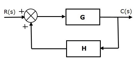
3.1 Positive Feedback
Here the feedback output is added to the desired input.
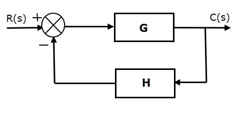
3.2 Negative Feedback
Here the feedback output is subtracted from the desired input. Negative feedback is used to reduce the error between the input and output.
4 Block Diagrams
4.1 Block Diagram Basics
4.1.1 Block
Blocks represent the transfer function of a component, with a single input and output.
The diagram below shows a block with input X(s), output Y(s) and transfer function G(s).

$$G(s) = \frac{Y(s)}{X(s)}$$
The output is obtained by multiplying the transfer function and input.
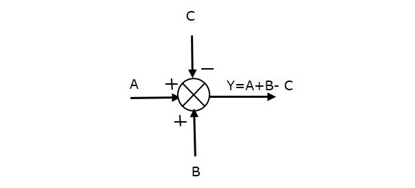
4.1.2 Summing Point
Represented by a circle, it receives 2 or more inputs and a single output. It is used to perform algebraic operation (summation and/or subtraction) on inputs to produce the operations result as an output. The operations on the inputs depend on their polarity.
The figures below shows a summing point and operations on inputs.
Recommended video: Basics of Block DIagrams
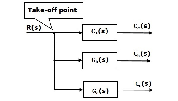
4.1.3 Taking-off point
This is a point on a branch from which an input/output can be passed to a summing point or one or more blocks.
4.2 Block Diagram Algebra
The multiple rules of block diagram algebra are shown below.
Recommended video: Block Diagram Algebra Rules
4.3 Block Diagram Reduction
The video provides an example on block diagram reduction.
Recommended video: Block Diagram Reduction Example
5 Transfer Functions
A transfer function represents the ratio of the laplace transform of a systems output signal and laplace transform of the systems input signal. Transfer functions can be obtained through reduction of a systems block diagram.
$$G(s) = \frac{Y(s)}{X(s)}$$
5.1 Poles and Zeros of Transfer Functions
A transfer function can be represented as:
$$G(s) = \frac{Y(s)}{X(s)} = K\frac{(s-z_1)(s-z_2)(s-z_n)} {(s-p_1)(s-p_2)( s-p_n)}$$
K is the gain factor of the transfer function.
From the equation if, s = $z_1$ or s = $z_2$ or s = $z_n$, the transfer function would become zero. Therefore, $z_1$, $z_2$ and $z_n$ are the zeros of the transfer function.
Now if, s = $p_1$ or s = $p_2$ or s = $p_n$, the transfer function would become infinite. Therefore, $p_1$, $p_2$ and $p_n$ are the roots of the transfer function.
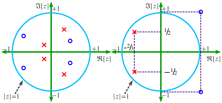
5.2 The S-Plane
The s-plane is a complex plane with a real and imaginary axis. The position on the complex plane is defined by $re^{j\theta}$ and the angle from the positive real axis, $\theta$. Poles are mapped on the s-plane as an x, while zeros are mapped as an o.

Recommended video: Introduction to Transfer Functions
5.3 Obtaining Transfer Function from a Block Diagram
Recommended video: Transfer Function from Block Diagram Reduction Example
5.4 MATLAB Implementation
Recommended video: Transfer function model
6 Time Response Analysis
The output response of a system varying with time is the time response of the system. The time response of a system consists of a transient state and steady state. Below is a generic time response of a system with the 2 states.
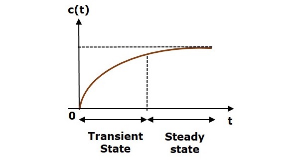
Mathematically a systems response c(t) is written as:
$$c(t) = c_{tr}(t) + c_{ss}(t)$$
6.1 Transient State Response
This state encompasses a systems output response until it reaches a steady state. For large values of time t, the transient response will be zero.
6.2 Steady State Response
This state refers to the steady section of a systems response where the transient response reaches a zero value, as t approaches infinity.
6.3 Standard Test Signal
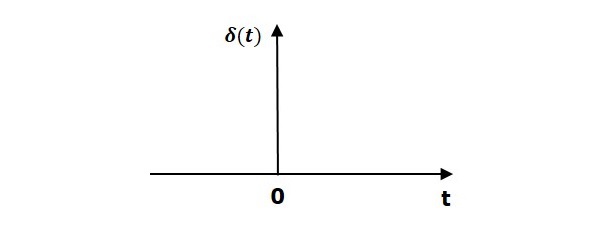
6.3.1 Unit Impulse Signal
Mathematically a unit impulse, $\delta$ is defined as:
$$\delta = 0;~t\neq0$$
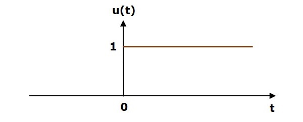
6.3.2 Unit Step Signal
Mathematically a unit step signal, u(t) is defined as:
$$u(t) = 1;~t\geq0$$
$$~~~~~= 0;~t<0$$
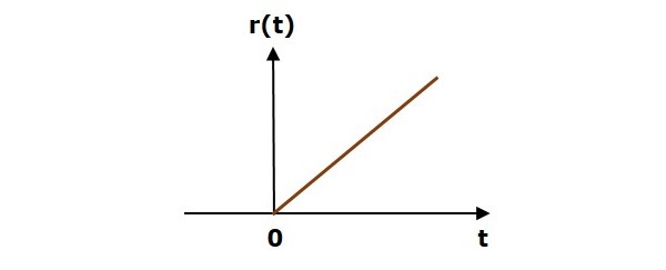
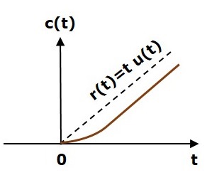
6.3.3 Unit Ramp Signal
Mathematically a unit step signal, r(t) is defined as:
$$r(t) = t;~t\geq0$$
$$~~~~~= 0;~t<0$$
7 Response of A First Order System
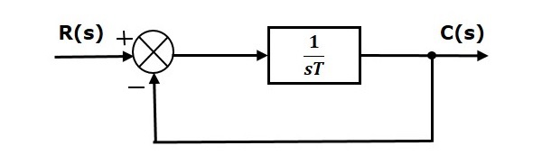
From the first order system above, the transfer function is:
$$\frac{C(s)}{R(s)} = \frac{G(s)}{1 + G(s)}$$
Substituting the value of G(s):
$${C(s)} = \frac{1}{sT + 1}{R(s)}$$
- C(s) is the laplace transform of output signal c(t).
- R(s) is the laplace transform of input signal R(t).
- T is the time constant.
For the time response of the output, the inverse laplace transform of the transfer function is performed.
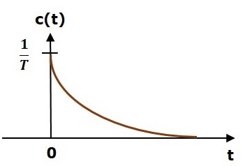
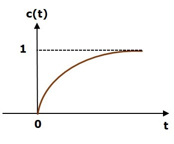
The table below shows the time domain responses to various signals. The constant values of the responses are the steady state components, while the transient components posses exponents.
| Signal | Response, c(t) |
|---|---|
| Unit impulse | $$c(t) = \frac{1}{T}e^{\frac{-1}{T}}u(t)$$ |
| Unit Step | $$c(t) = (1-e^{\frac{-1}{T}})u(t)$$ |
| Unit Ramp | $$c(t) = (t-T-Te^{\frac{-1}{T}})u(t)$$ |
Unit Impulse Response
Unit Step Response
Unit Ramp Response
8 Response of A Second Order System
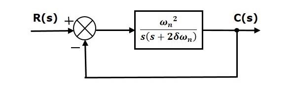
From the second order system above, the transfer function is:
$$C(s) = (\frac{w_n^2}{s^2+2\zeta w_n s+w_n^2})R(s)$$
- C(s) is the laplace transform of output signal c(t).
- R(s) is the laplace transform of input signal R(t).
- $w_n$ is the natural frequency: The oscillation frequency of a system which is disturbed and then allowed to oscillate freely.
- $\zeta$ is the damping ratio: Quantity that describes the damping level in a system.
For the time response of the output, the inverse laplace transform of the transfer function is performed.
The table below shows the time domain responses to a unit step signal, under different ranges of $\zeta$.
| Damping ratio, $\zeta$ | Response, c(t) | Response Type |
|---|---|---|
| $\zeta = 0$ | $$c(t) = (1-\cos{w_n t})u(t)$$ | Undamped |
| $\zeta = 1$ | $$c(t) = (1-e^{-w_n t}-w_n te^{-w_n t})u(t)$$ | Critically Damped |
| $0<\zeta<1$ | $$c(t) = (1- (\frac{e^{-\zeta w_n t}}{\sqrt{1-\zeta^2}})(\sin{w_d t + \theta})u(t)$$ | Underdamped |
| $\zeta > 1$ | $$c(t) = (1+(\frac{1}{2(\zeta+\zeta^2-1)})e^-(\zeta w_n+ w_d)t-(\frac{1}{2(\zeta-\zeta^2+1)})e^-(\zeta w_n-w_d)t)$$ | Overdamped |
- $w_d$ is the damping frequency: This quantity is mathematically defined as:
$$w_d = w_n \sqrt{1 - \zeta^2}$$
9 Time Domain Specifications of a 2nd Order System
Response of a 2nd order underdamped system.
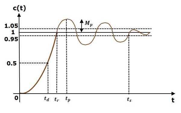
9.1 Delay Time
Delay time $t_d$, is the required time for an underdamped system response to reach half of its final value, from it zero instance.
9.2 Rise Time
This is the time $t_r$, taken for an underdamped system response to rise from 0% to 100% of its final value. For an overdamped system response, it is the time to rise from 0% to 100% of its final value.
The quantity is defined mathematically below:
$$t_r = \frac{\pi - \tan^{-1}(\frac{\sqrt{1-\zeta^2}}{\zeta})}{w_n \sqrt{1-\zeta^2}}$$
9.3 Peak Time
Peak time $t_p$ is the time taken for a response to reach its maximum value for the first time.
The quantity is defined mathematically below:
$$t_P = \frac{\pi}{w_d}$$
9.4 Peak Overshoot
Overshoot $M_p$ is the deviation of the systems response from the final steady state response at peak time.
The quantity is defined mathematically below:
$$M_p = (e^-(\frac{\zeta \pi}{\sqrt{1-\zeta^2}}))$$
The percentage of peak overshoot can be found from the above equation.
9.5 Settling Time
This is the time $t_s$ taken for a response to reach its steady state final value and remain within a specific tolerance range of the value.
For a 2% tolerance range, the quantity is defined mathematically below as:
$$t_s = \frac{4}{\zeta w_n} = 4\tau$$
- $\tau$ is the time constant: This is the time taken for a response to reach 63.2% of its final steady state value from the initial state.
Recommended video: Time Domain Specifications
10 Steady State Error
This refers to the discrepancy between a control systems output from the desired steady state response.
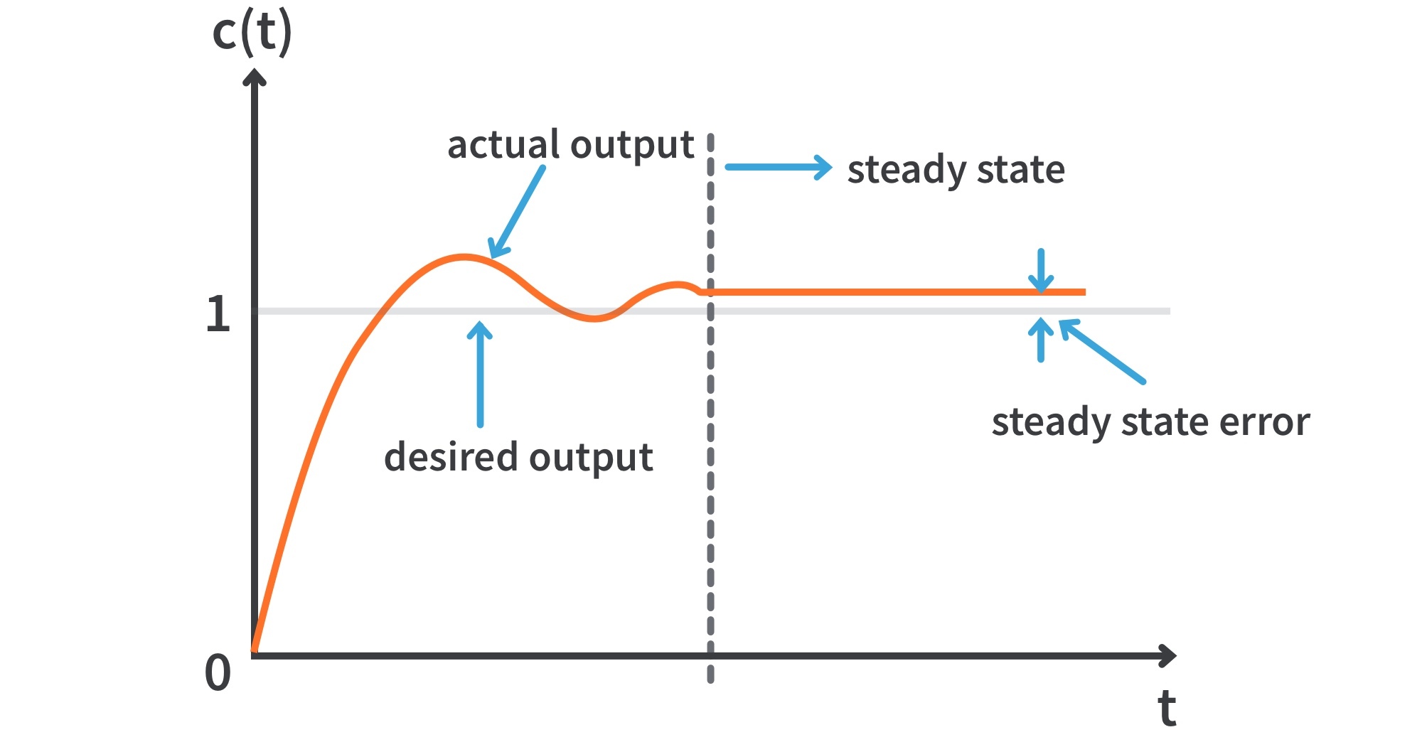
The quantity is defined mathematically below as:
$$e_{ss} = \lim_{x\to\infty} e(t) = \lim_{s\to 0} sE(s)$$
- E(s) is the laplace transform of signal, e(t).
Recommended video: Steady State Error
11 Stability
For a stable system produces a bounded output for a given bounded input.
11.1 Types of Stability
The classification of systems based on stability is given below.
- Absolutely Stable System: This system provides bounded output for all variations in the system. If all the poles of the open loop and closed loop transfer function is on the left half of the s-plane, then the open and closed loop control system is absolutely stable.

- Conditionally Stable System: Here the system provides bounded output for only a range of variations in the system.

- Marginally Stable System: This system produces bounded output when the bounded input possess constant amplitude and frequency. If any 2 poles of the open loop and closed loop transfer function is on the imaginary of the s-plane, then the open and closed loop control system is marginally stable.

- Unstable Stable System: This system provides unbounded output for all variations in the system. If all the poles of the open loop and closed loop transfer function is on the right half of the s-plane, then the open and closed loop control system is absolutely stable.

Recommended video: Introduction to Stability
12 Frequency Response
Frequency response is the response of a system for a given sinusoidal input.
For an input signal $r(t) = A\sin(\omega_0 t)$ and open loop transfer function $G(s) = G(j\omega)$, with magnitude and phase $G(j\omega_0)|\angle G( j\omega_0)|$ the output signal is:
$$c(t) = A|G(j\omega_0)|\sin(\omega_0 t+\angle G(j\omega_0))$$
-
A is the amplitude of the input signal.
-
$\omega_0$ is the angular frequency of the input signal, mathematically described as: $$\omega_0 = 2\pi f_0$$
-
$f_0$ is the frequency of the input signal.
13 Frequency Domain Specifications
For the 2nd order transfer function:
$$T(S) = \frac{C(s)}{R(s)} = (\frac{w_n^2}{s^2+2\zeta w_n s + w_n^2})$$
The magnitude of T(s), with $s = j\omega$:
$$M = |T(j\omega)| = \frac{1}{\sqrt{(1-(\frac{\omega}{\omega_n})^2)^2+(2\zeta \frac{\omega}{\omega_n})^2}}$$
The phase of T(s), with $s = j\omega$:
$$\angle T(j\omega) = -\tan^{-1}(\frac{\frac{2\zeta\omega}{\omega_n}} {1 - ( \frac{\omega}{\omega_n})^2})$$
13.1 Resonant Frequency
Resonant frequency, $\omega_r$, is the frequency when the magnitude of the frequency response reaches its peak value for the first time.
It is mathematically defined as:
$$\omega_r = \omega_n\sqrt{1-2\zeta^2}$$
13.2 Peak Resonance
Peak resonance, $M_r$ is the maximum magnitude of $T(j\omega$).
It is mathematically defined as:
$$M_r = \frac{1}{2\zeta\sqrt{1-\zeta^2}}$$
13.3 Bandwidth
Bandwidth, $\omega_b$, is the frequency range over which, the magnitude of $T( j\omega$) drops to 70.7% of its zero frequency value.
$$\omega_b = \omega_n\sqrt{1-2\zeta^2 + \sqrt{2-4\zeta^2+4\zeta^4}}$$
14 Control System Plots
14.1 Bode Plot
Bode Plots describe the change in magnitude and phase as a function of frequency.
The magnitude of an open loop transfer function in dB is:
$$M = 20\log(|G(j\omega)H(j\omega)|)$$
The phase angle of an open loop transfer function in degrees is:
$$\phi = \angle G(j\omega)H(j\omega)$$
Recommended video: Introduction to Bode Plots
Recommended video: Bode Plot Solved Example
14.1.1 Stability Analysis with Bode Plots
14.1.1.1 Cross Over Frequency
- Phase Cross Over Frequency, $\omega_pc$: This is the frequency at which the bode phase plot has a phase of $-180^\circ$. Its unit is rad/sec.
- Gain Cross Over Frequency, $\omega_gc$: This is the frequency at which the bode magnitude plot has a magnitude of zero dB. Its unit is rad/sec.
| Stability Criteria | Stability |
|---|---|
| $\omega_pc > \omega_gc$ | Stable system |
| $\omega_pc = \omega_gc$ | Marginally Stable system |
| $\omega_pc < \omega_gc$ | Unstable system |
14.1.1.2 Gain and Phase Margin
- Gain Margin, GM: This is the negative value of magnitude in dB at the phase cross over frequency, $M_pc$.
It is mathematically defined as:
$$GM = 20\log(\frac{1}{M_pc}) = 10\log(M_pc)$$
- Phase Margin, PM: It is mathematically defined as:
$$PM = 180^\circ + \phi_gc$$
where $\phi_gc$, is the phase angle at the gain cross over frequency.
| Stability Criteria | Stability |
|---|---|
| $GM > 0$ and $PM > 0$ |
Stable system |
| $GM = 0$ and $PM = 0$ |
Marginally Stable system |
| $GM < 0$ and/or $PM < 0$ |
Unstable system |
Recommended video: How to find cross over frequencies, Gain and Phase Margin from Bode Plot
14.1.2 MATLAB Implementation
Recommended video: Bode plot of frequency response, or magnitude and phase data
14.2 Nyquist Plot
14.2.1 Nyquist Stability Criterion
The criterion states that if P poles and Z zeros are encircled by an enclosed path in the s plane, the corresponding G(s)H(s) plane must encircle the origin P-Z times. The encirclement number, N, is given by:
$$N = P - Z$$
- If only poles exist in the encircled s plane closed path, the encirclement in the G(s)H(s) is opposite in direction to the path in the s plane.
- If only zeros exist in the encircled s plane closed path, the encirclement in the G(s)H(s) is in the same direction as the path in the s plane.
The Nyquist Stability Criterion states that N of the point (-1,0) must equal P-Z of the close loop transfer function.
Recommended video: Nyquist plot intro 1
Recommended video: Nyquist plot intro 2
14.2.2 Stability Analysis with Nyquist Plots
14.2.1.1 Cross Over Frequency
- Phase Cross Over Frequency, $\omega_pc$: This is the frequency at which the Nyquist plot intersects the negative real axis (phase of $-180^\circ$). Its unit is rad/sec.
- Gain Cross Over Frequency, $\omega_gc$: This is the frequency at which the Nyquist plot has a magnitude of 1. Its unit is rad/sec.
| Stability Criteria | Stability |
|---|---|
| $\omega_pc > \omega_gc$ | Stable system |
| $\omega_pc = \omega_gc$ | Marginally Stable system |
| $\omega_pc < \omega_gc$ | Unstable system |
14.2.1.2 Gain and Phase Margin
- Gain Margin, GM: This is the reciprocal value of magnitude at the phase cross over frequency, $M_pc$.
It is mathematically defined as:
$$GM = \frac{1}{M_pc}$$
- Phase Margin, PM: It is mathematically defined as:
$$PM = 180^\circ + \phi_{gc}$$
where $\phi_gc$, is the phase angle at the gain cross over frequency.
| Stability Criteria | Stability |
|---|---|
| $GM > 1$ and $PM > 0$ |
Stable system |
| $GM = 1$ and $PM = 0$ |
Marginally Stable system |
| $GM < 1$ and/or $PM < 0$ |
Unstable system |
Recommended video: How to find cross over frequencies, Gain and Phase Margin from Nyquist Plot
14.2.3 MATLAB Implementation
Recommended video: Nyquist plot of frequency response
15 State Space
- State: A group of variables which summarize the systems history, utilized to predict future outputs.
- State Variables: They possess the dynamic information of a system.
The state space model of a linear time invariant system is represented as:
-
State Equation: $$\dot {X} = AX + BU$$
-
Output Equation: $$Y = CX + DU$$
- X and $\dot {X}$, are the state vector and differential state vector.
- Y and U, are the output and input vectors.
- A is the system matrix.
- B and C are the input and output matrices.
- D is the feed forward matrix.
Applying laplace transform to the state space model defined above, the transfer function of a system in state space is defined as:
$$\frac{Y(s)}{U(s)} = C(sI-A)^{-1}$$
- I is an identity matrix.
15.1 State Transition Matrix
If the matrix satisfies the following linear homogenous equation:
$$\dot x(t) = \frac{dx(t)}{dt} = Ax(t)$$
The state transition matrix $\phi (t)$ is:
$$\frac{d\phi (t)}{dt} = A\phi (t)$$
The condition following will be met:
$$x(t) = \phi (t)x(0)$$
Taking laplace of the linear homogenous equation:
$$x(t) = \phi (t)x(0) = L^{-1}[(sI - A)^{-1} x(0)]$$
Properties of State Transition Matrix:
- $\phi (t) = I$
- $\phi (t) = e^{At} = (e^{-At})^{-1} = (\phi (-t))^{-1}$
- $\phi (t_2 - t_0) = \phi (t_2 - t_1)\phi(t_1 - t_0)$
- $\phi (t - t_0) = \phi (t)\phi^{-1} (t_0)$
- $\phi (t+t_0) = \phi (t)\phi(t_0)$
15.2 Controllability and Observability
- Controllability: A system is controllable when a desired output is obtained from a specified and controlled input. The criteria is given below, using the matrix $Q_0$.
$$Q_0 = [B AB A^2B .... A^{n-1}B]$$
If the determinant of $Q_0$, $|Q_0|$ is unequal to 0, then the system is controllable.
- Observability: If input and output signals are used to determine the internal state of a system within a finite interval of time, the system is observable. The criteria is given below, using the matrix $Q_0$.
$$Q_0 = [C^T A^T C^T .... (A^T)^{n-1}C^T]$$
If the determinant of $Q_0$, $|Q_0|$ is unequal to 0, then the system is observable.
Recommended videos:
- Introduction to State-Space Equations | State Space, Part 1
- What is Pole Placement (Full State Feedback) | State Space, Part 2
- A Conceptual Approach to Controllability and Observability | State Space, Part 3
- What Is Linear Quadratic Regulator (LQR) Optimal Control? | State Space, Part 4
- State Space Models, Part 1: Creation and Analysis
- State Space Models, Part 2: Control Design
16 code implementations
Recommended video: 4 Ways to Implement a Transfer Function in Code | Control Systems in Practice
17 Applications & Design
Recommended videos: PID Controller Implementation in Software - Phil's Lab #6 Introduction - Control System Design 1/6 - Phil's Lab #7 Modelling of Dynamical Systems - Control System Design 2/6 - Phil's Lab #8 System Identification with Matlab - Control System Design 3/6 - Phil's Lab #9